In DFT Basics : Article #18, we had explored Fault Simulation and Stuck at Fault Model. In this post, we will explore Transition Delay Fault (TDF) Model.
Let’s get started !
Transition Delay Fault Model
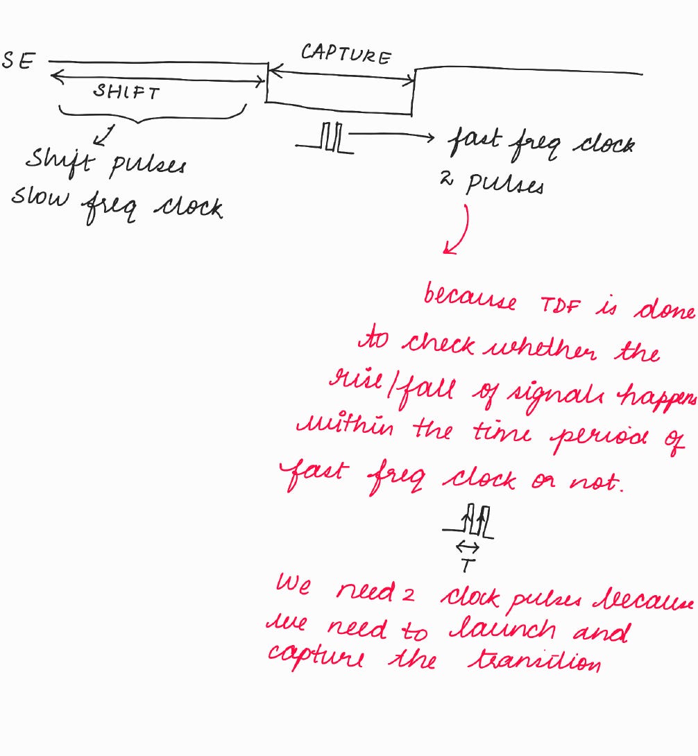
TDF fault model is used to detect that the logic level from 0-1 and 1-0 properly transit within the specific time (time period of fast frequency clock (i.e., functional clock)) or not.
Why fast frequency clock?
Because after manufacturing (i.e., after testing when the chip goes to the customer), only fast frequency clock (i.e., functional clock) will be used. So we need to check whether the rise/fall of signals happens within the time period of fast frequency clock or not.
< < We have explored how the appropriate clock and appropriate no. of clock pulses are propagated in DFT Basics : Article #14> >
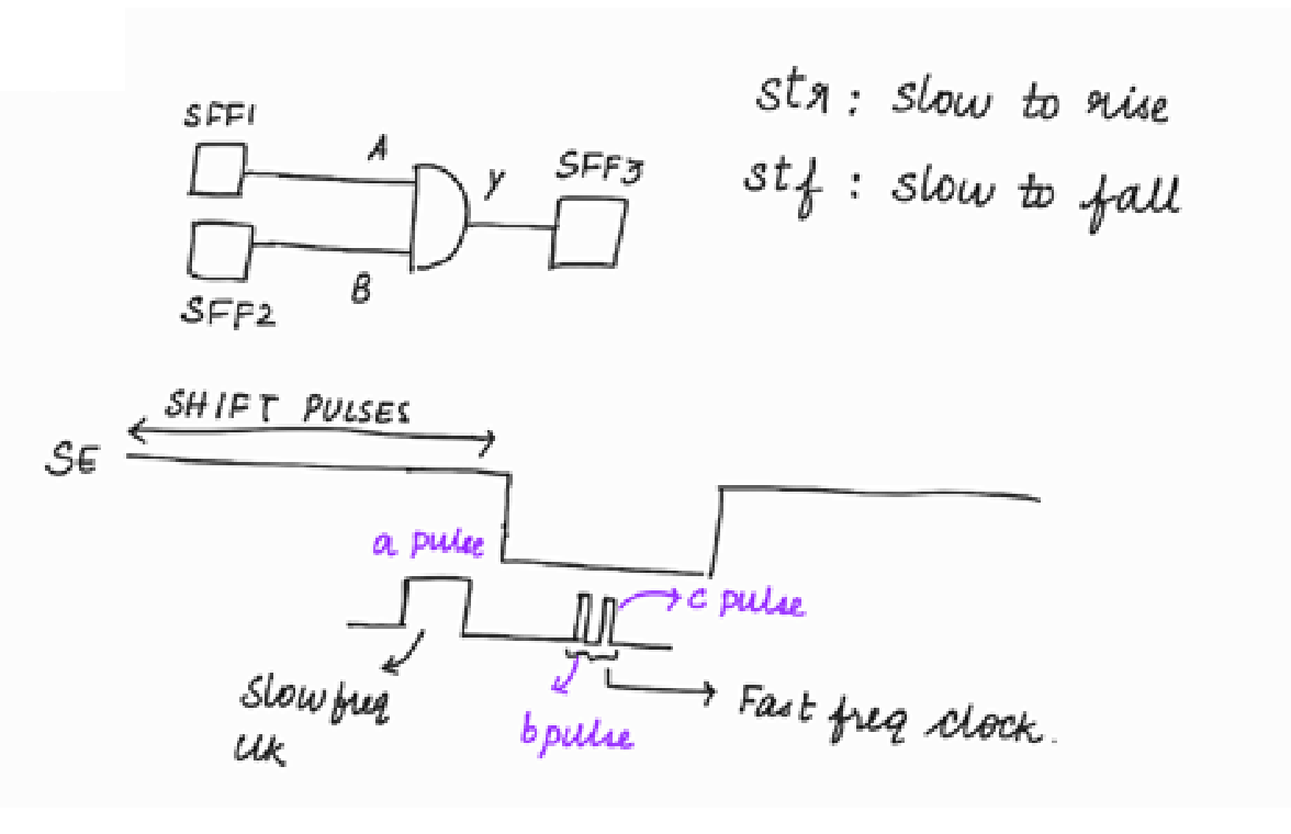
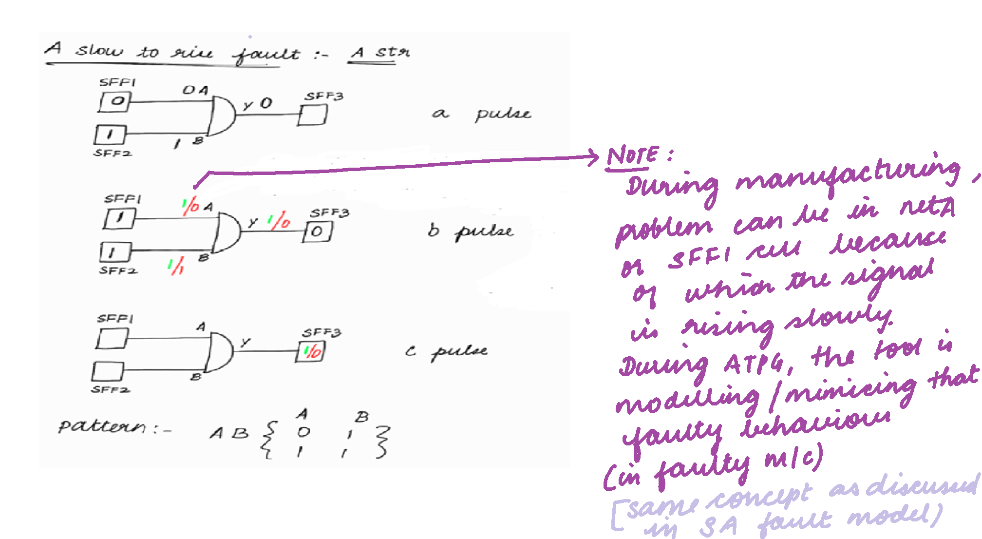
Let’s explore more on TDF using the below example :
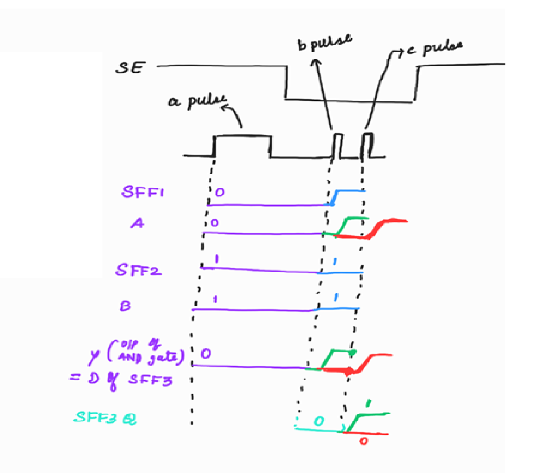
Let’s explore the same using a waveform:
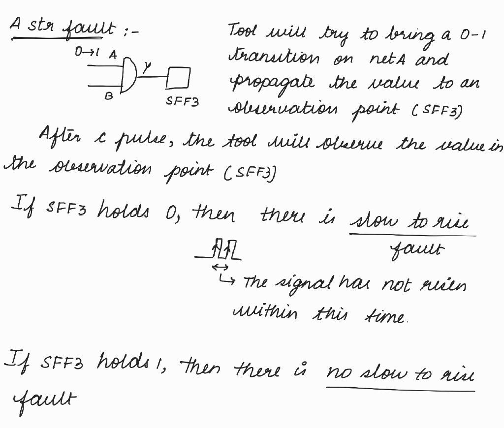
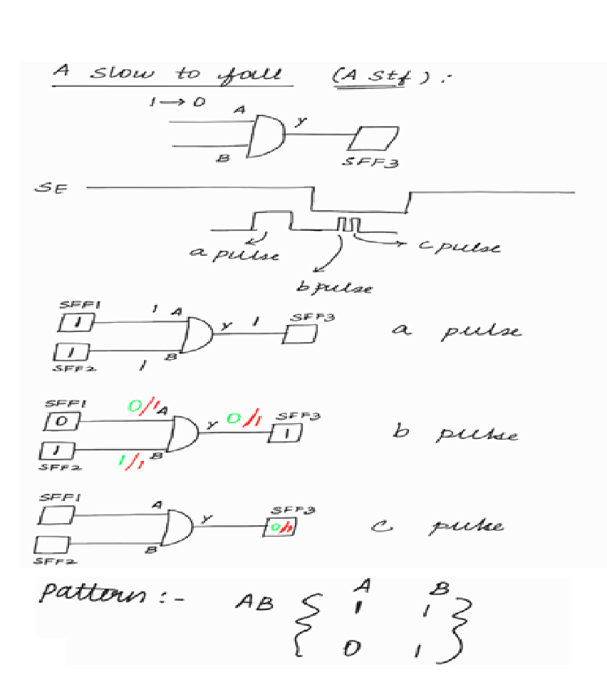
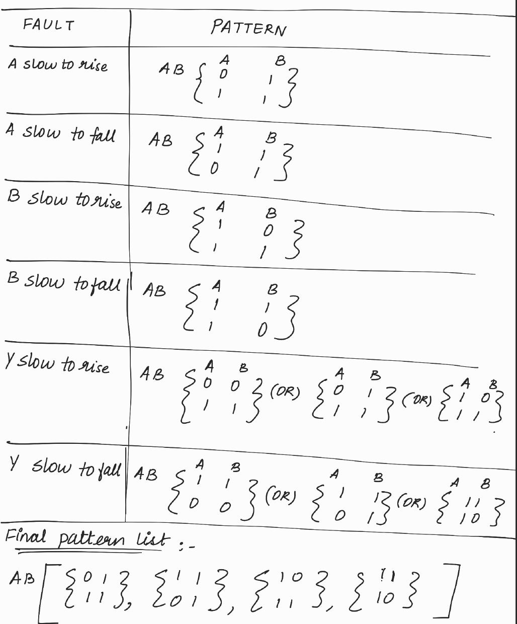
The same concept is applied to the other faults and I have arrived at the below tabular column
< < Note : Tool will not write the redundant patterns into the final pattern list > >
Ways to detect TDF faults
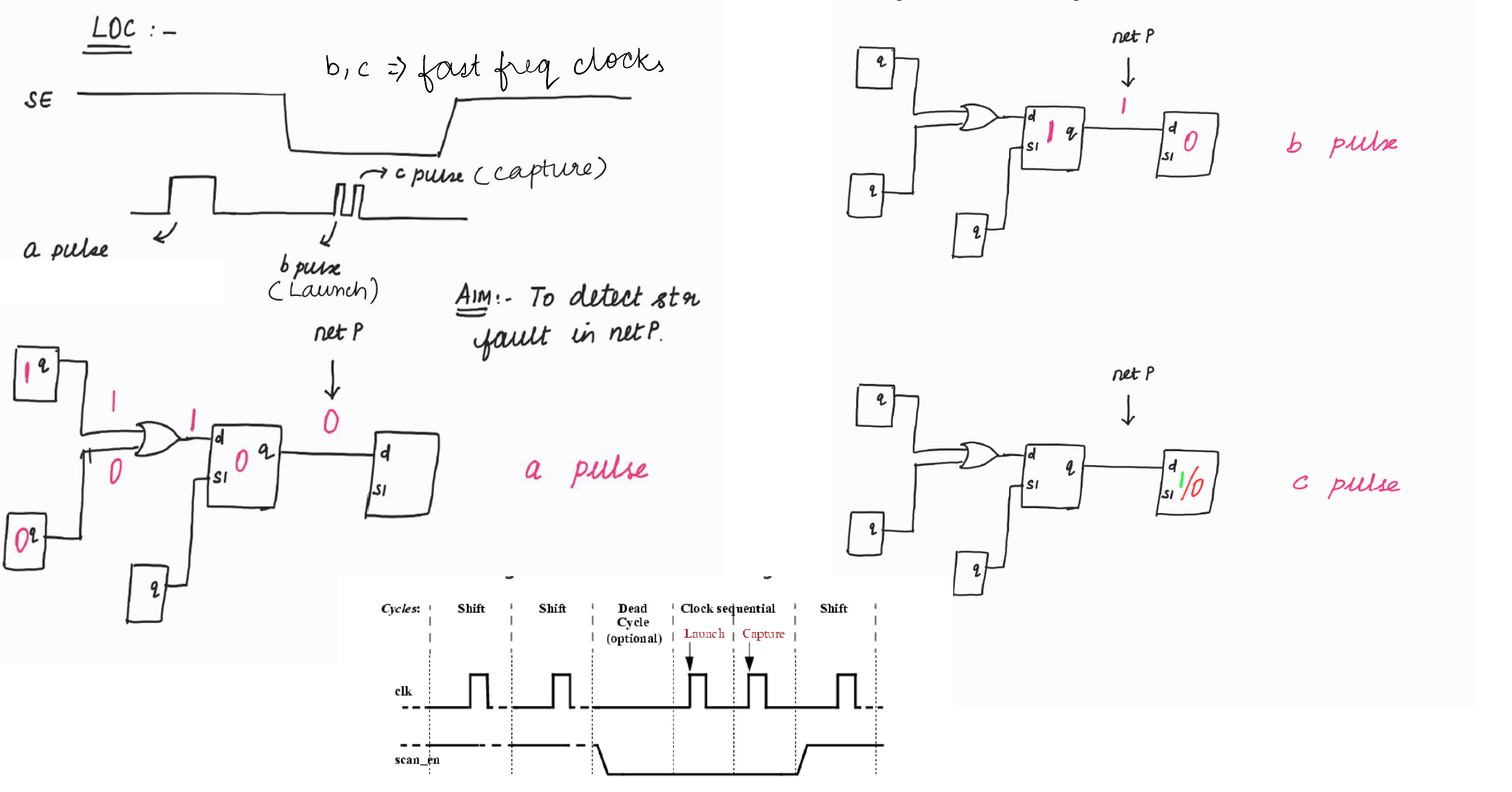
LOC : Launch on Capture (or) Launch off Capture
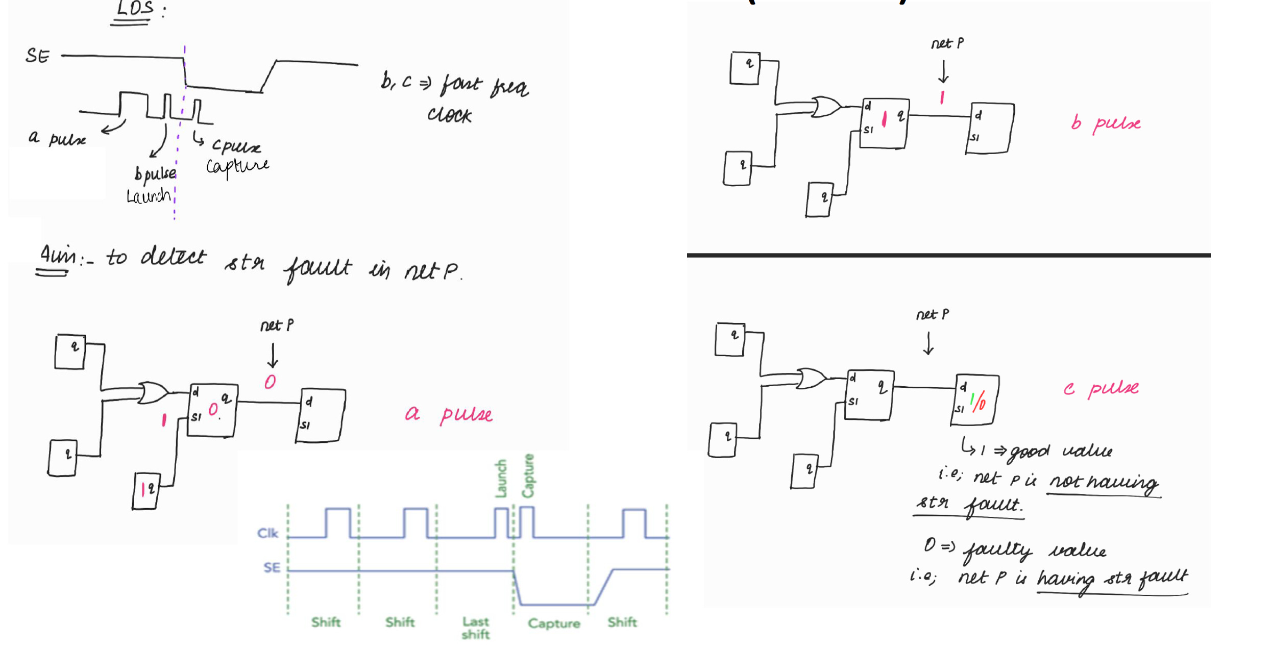
LOS : Launch on Shift (or) Launch off Shift
LOC : Launch on Capture (or) Launch off Capture
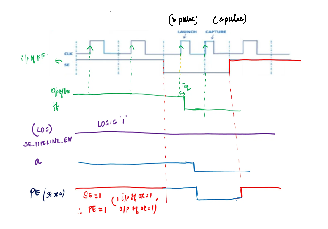
LOS : Launch on Shift (or) Launch off Shift In LOS, the launch pulse (i.e., b pulse in our waveforms) will come during SEN=1 and it will be the last shift pulse.
Comparison:
LOS has slightly more coverage compared to LOC as the tool has more controllability on LOS than LOC.
Explanation:
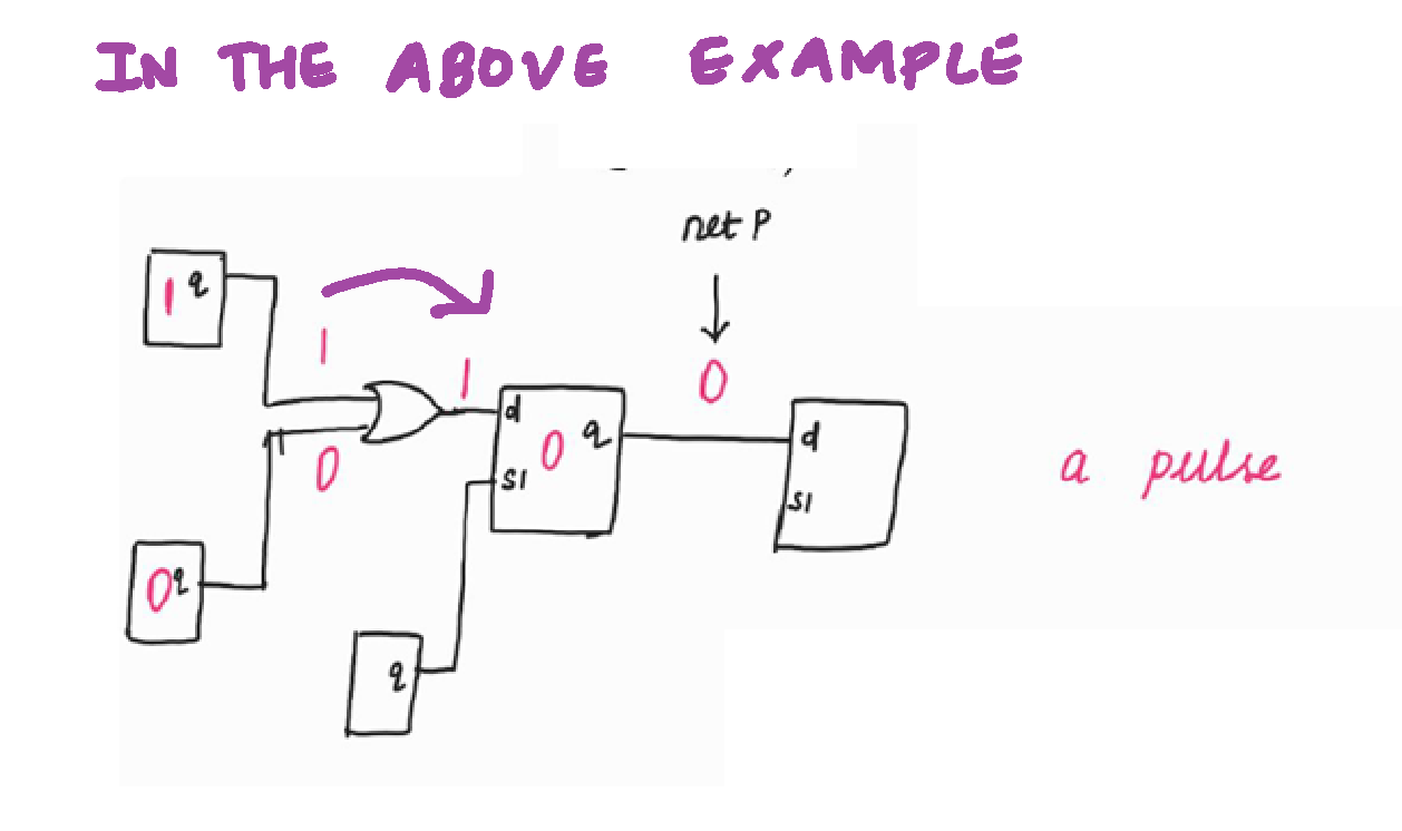
The tool brings the transition value through shift path in LOS (as depicted with the arrow in the below figure).
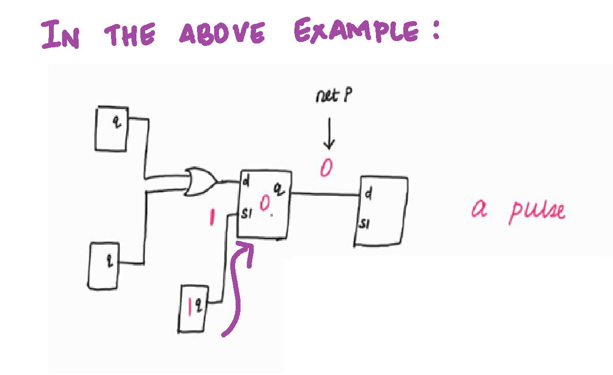
Whereas in LOC, the tool has to program the combo logic to get an appropriate value at the output of the combo logic to create the transition (as depicted with an arrow in the below figure). Suppose the tool is not able to bring the appropriate value at the output of combo logic, then the faults that require that value will not get detected.
But there is a major limitation in LOS. Controlling SE (timing closure on SE) is extremely difficult. Therefore mostly companies don’t use LOS.
As per the OCC’s internal architecture, when Scan Enable (SE) = 1, both for SA and TDF, slow frequency clock is propagated. How while using LOS method, we are able to propagate 1 fast frequency clock (b pulse in our waveforms) during SE = 1 ?
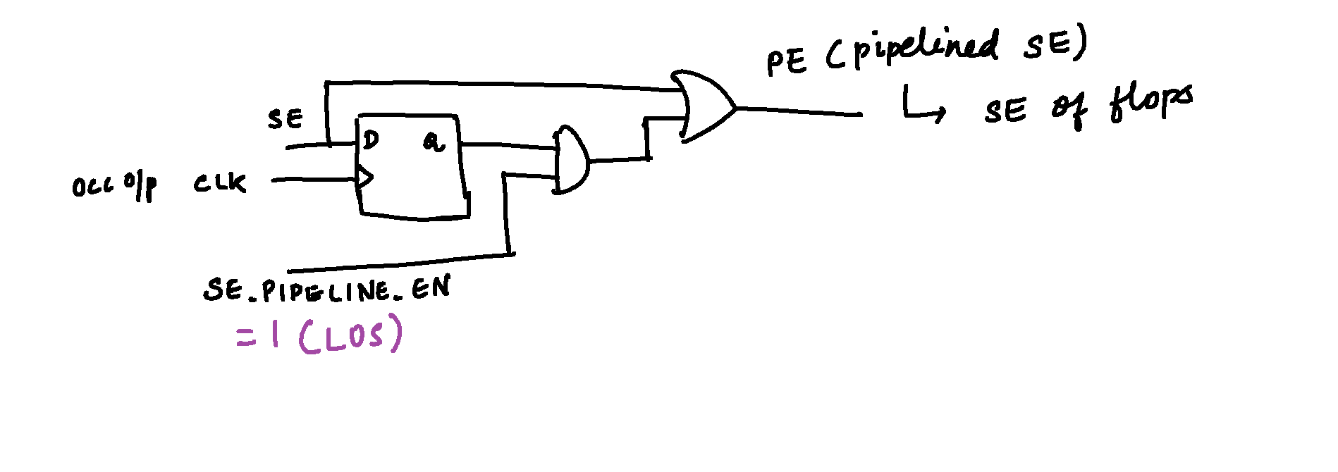
Ans : Using Pipelined Scan Enable (PSEN)
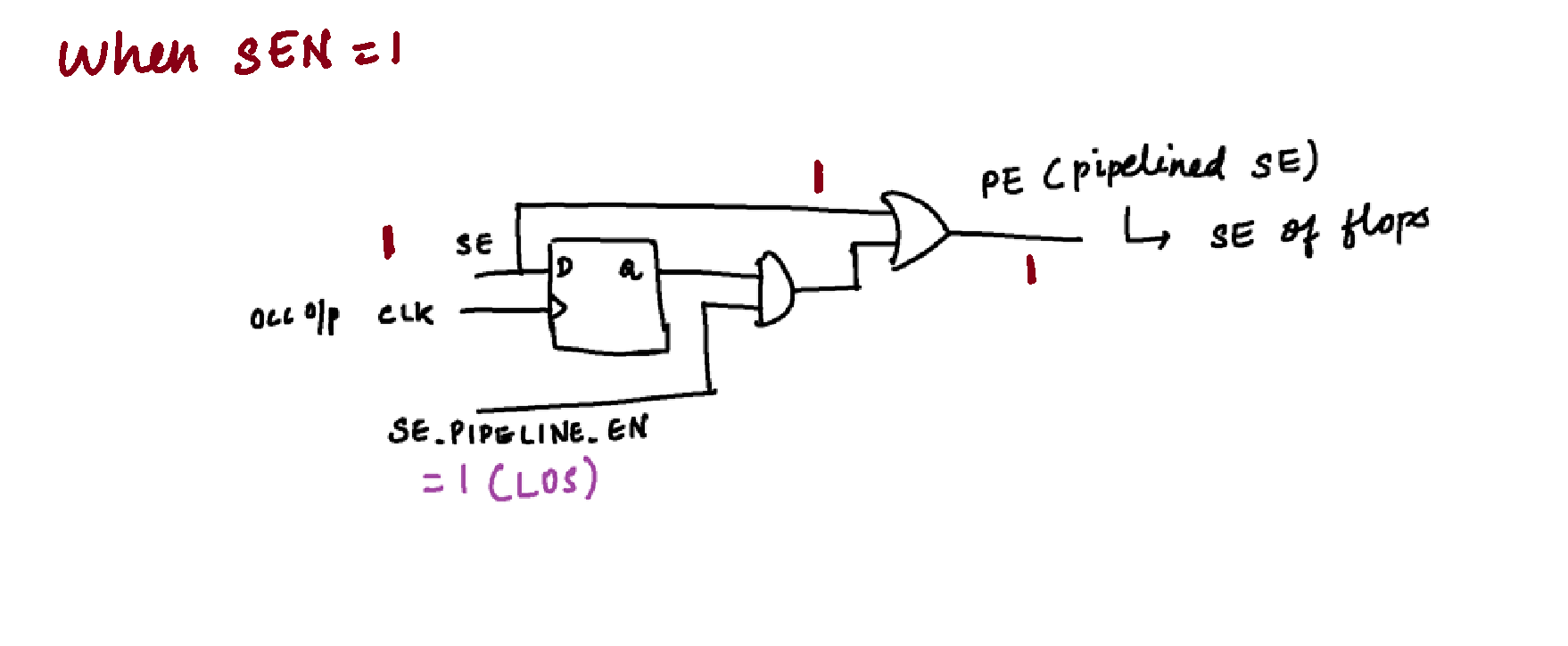
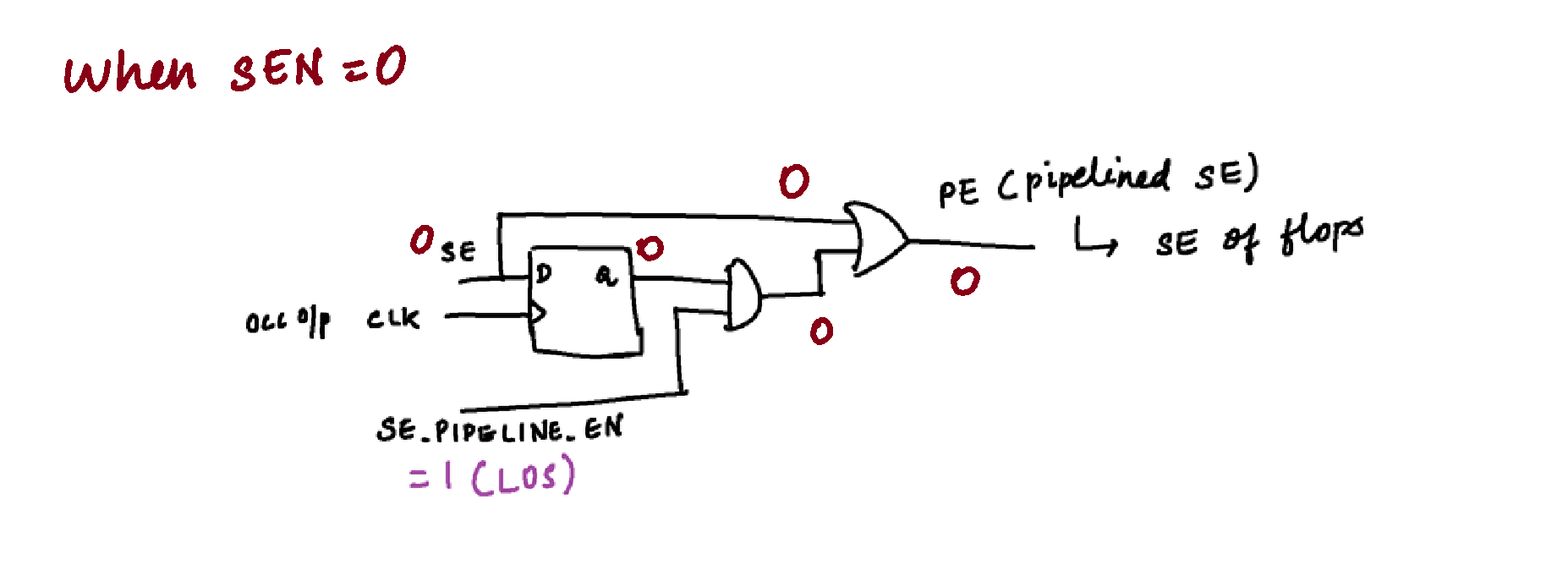
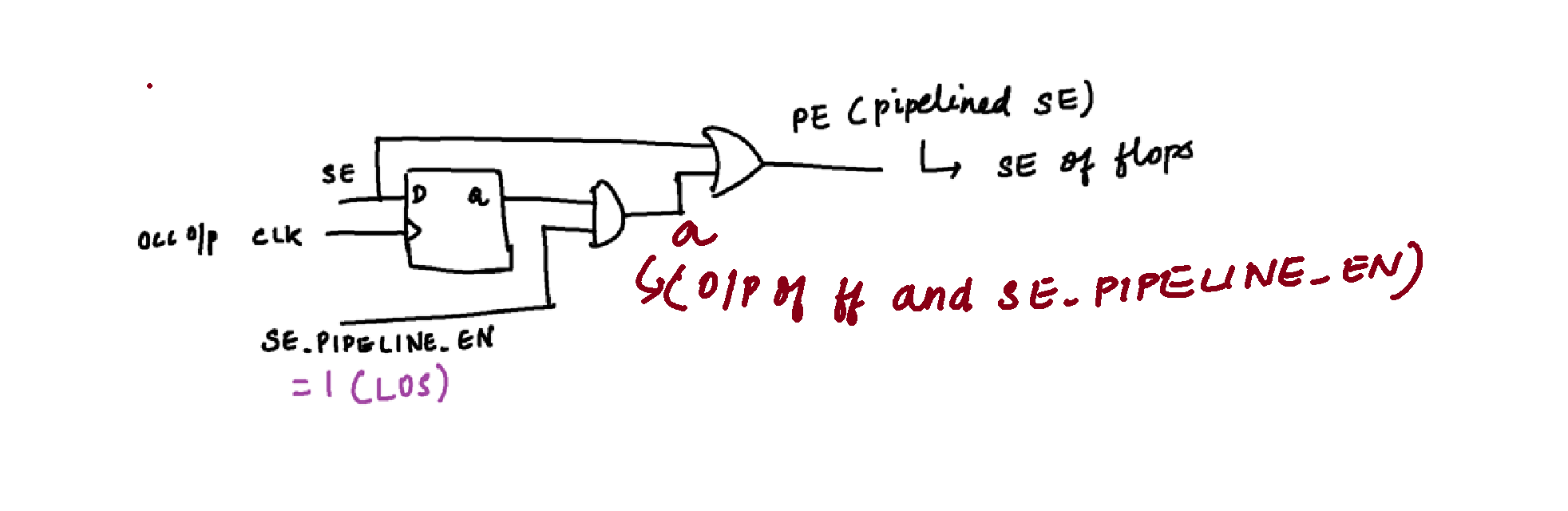
Now let’s explore the PSEN architecture.
Let’s visualize the above diagrams using a waveform :
< < Note : In the above waveform Tcq is the clock to q delay > >
In this post, we had explored Transition Delay Fault (TDF) Model, ways to detect TDF and PSEN architecture. In the next post, we will explore Path Delay Fault (PDF) Model. We will discuss the necessity of having both PDF and TDF.